
Full series: capacity modelling guide
In part 1 of this series, we discussed the data that is needed for capacity modelling and the use of a trend of historical resource data, where forecasts of business data are not forthcoming. The initial step to developing this type of forecast was to analyse the historical resource data to ensure that a trend could be identified.
Following on from that, this blog will describe how to generate the capacity forecast, using the historical component data. A trend essentially involves drawing a straight line through the historical data and then using the inclination of this straight line to determine the forecast values into the future. Microsoft Excel has built-in Regression analysis functionality, which allows you to determine the gradient and intercept of the straight line. This may not be enabled in your Microsoft Excel installation by standard. To activate it, follow these steps in Microsoft Excel 2010:
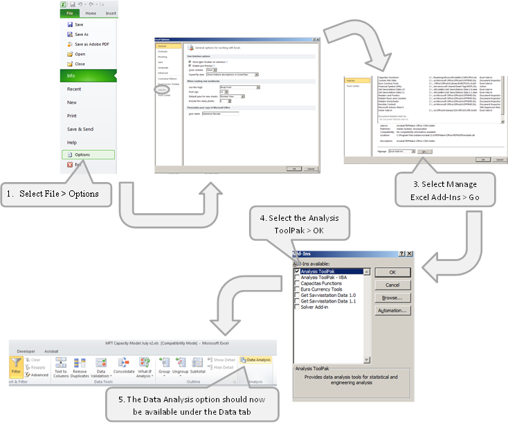
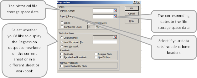
Selecting Data Analysis from the toolbar then allows you to perform various analytical methods on your data sets. One of these is “Regression”, which determines the relationship between two sets of variables. In our case, the tool will determine how the file storage space changes with time. The Regression tool requires the following inputs:
The output of the Regression analysis is as follows:
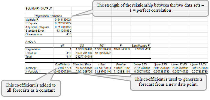
Alternatively, the Intercept can be determined using the in-built Microsoft Excel INTERCEPT function, where the same data sets are passed as arguments. Similarly, the “X Variable 1” Coefficient can be calculated using the SLOPE function and the R Square can be computed from the RSQ function.
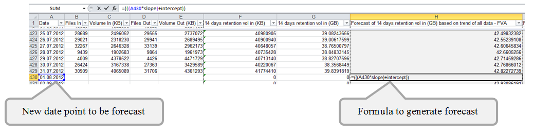
The two coefficients can then be used for generating a forecast of file storage space used on any future date using the following formula:
(<future date> x SLOPE) + INTERCEPT
In the screenshot below, the cell where the SLOPE and INTERCEPT have been calculated have been named as SLOPE and INTERCEPT for ease of reference:
That’s it for this week; by this point you should have forecast resource values based on the historical trend over time. For some of you, that might be all you need to achieve – and in that case, wasn’t it easy?! However, if you expect your model to be used by others and you want to make it more user-friendly and flexible with options for modelling various scenarios, watch out for the next part of this series.

