
In previous posts we looked a few simple ways to create forecasts in Excel, first using Time Series Decomposition, and also regression against business drivers.
The advantage of using business metrics is clear: if the business know what they are doing and are forecasting it we can use their forecasts to work out how busy our servers will be.
However often there are big differences between how the business do their forecasting and how you want to forecast for your servers. These will probably include differences in granularities and aggregations. The business forecast may be a number of anticipated trades per month, for example, while you need to know the peak hour of the busiest day
One solution to this is to carry out a form of Time Series Decomposition using the business forecast to drive the trend – it’s quite simple really and this tutorial will walk through the steps you need to carry out.
Get data
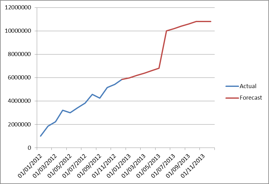
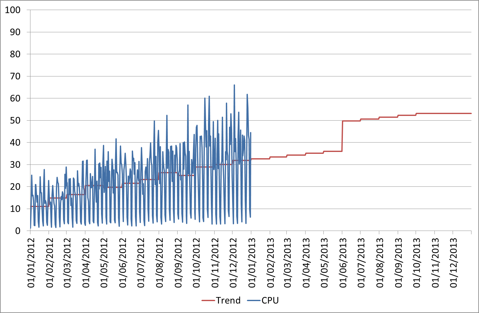
First of all get your historical and forecast business volumes, at the same granularity. In this example we have monthly values, as shown in the chart below. The business volumes handled by this part of the organisation have been growing fast since it was started at the beginning of the year; this year they will flatten off except for a large jump in June, maybe due to an acquisition or merger:
Verify Relationship
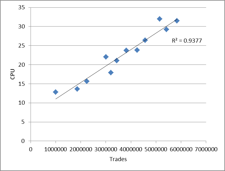
Next you should confirm that a good relationship exists by comparing to monthly average or total CPU. You can do this visually on an Excel scatter chart and by adding a trendline you also have the option to display the R2 figure. Here you can see we have a nice fit (the closer to 1 the R2 is the better).
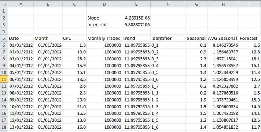
If the relationship is good enough then create a table like this (assuming you want to forecast daily CPU)
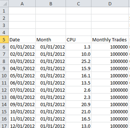
Here Date and CPU are self-explanatory and the Month column gives us the month for the date (using =DATE(YEAR(A6),MONTH(A6),1)). The Monthly Trades uses the Month column to lookup against the table (in a separate sheet named BusinessData) of monthly business volumes (actual and predicted): =VLOOKUP(B6,BusinessData!A:C,2,FALSE)
Create Trend
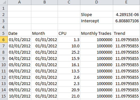
Now we are ready to create our trend. In Basic Time Series Decomposition in Excel we looked at how to do this based on date; what we are going to do here is just the same only based on Monthly Trades instead. We calculate the slope and intercept as
=SLOPE(C6:C371,D6:D371)
=INTERCEPT(C6:C371,D6:D371)
where as above column C contains the CPU, D the Monthly Trades. Then use these to calculate the Trend column as for instance =D6*E$2+E$3 where E$2 is the Slope and E$3 the Intercept, and, crucially, D6 is the monthly trades for that period.
The spreadsheet will now look like this:
And the Trend, compared to the actual CPU, will look like this:
Add Seasonality
Now just as we did before with Time Series Decomposition we want to add the seasonality in. I’ve introduced a couple of different variations this time to make it more interesting:
- Seasonal identifier which takes month profile into account as well as week
- Multiplicative decomposition rather than additive
First of all instead of just using the WEEKDAY() function to generate a seasonality identifier I’m using the following equation:
=INT((DAY(A6)/7)) & "_" & WEEKDAY(A6)
Basically what this is trying to do is take into account roughly which week of the month we are looking at as well, distinguishing between the week at the end of the month and the week at the start of the month. This may or may not be useful; the only point I’m making with this is that you can make up whatever identifier you like for the seasonality based on your understanding of the data. Try out some different combinations – for instance just using DAY() will give you day of month.
The other change is simple but makes a big difference – to get the Seasonal column now instead of subtracting the trend from the actual I’m dividing it (=C6/E6). Then instead of adding it back on in the Forecast I’m multiplying it back in (=E6*H6). Try out both methods and you’ll soon see the difference.
Here is a final view then of all the columns we need – remember AVG Seasonal is calculated as =SUMIF(F$6:F$371,F6,G$6:G$371)/COUNTIF(F$6:F$371,F6), the exact ranges depending on the date range you want to use for your seasonality. Here it’s the whole year.
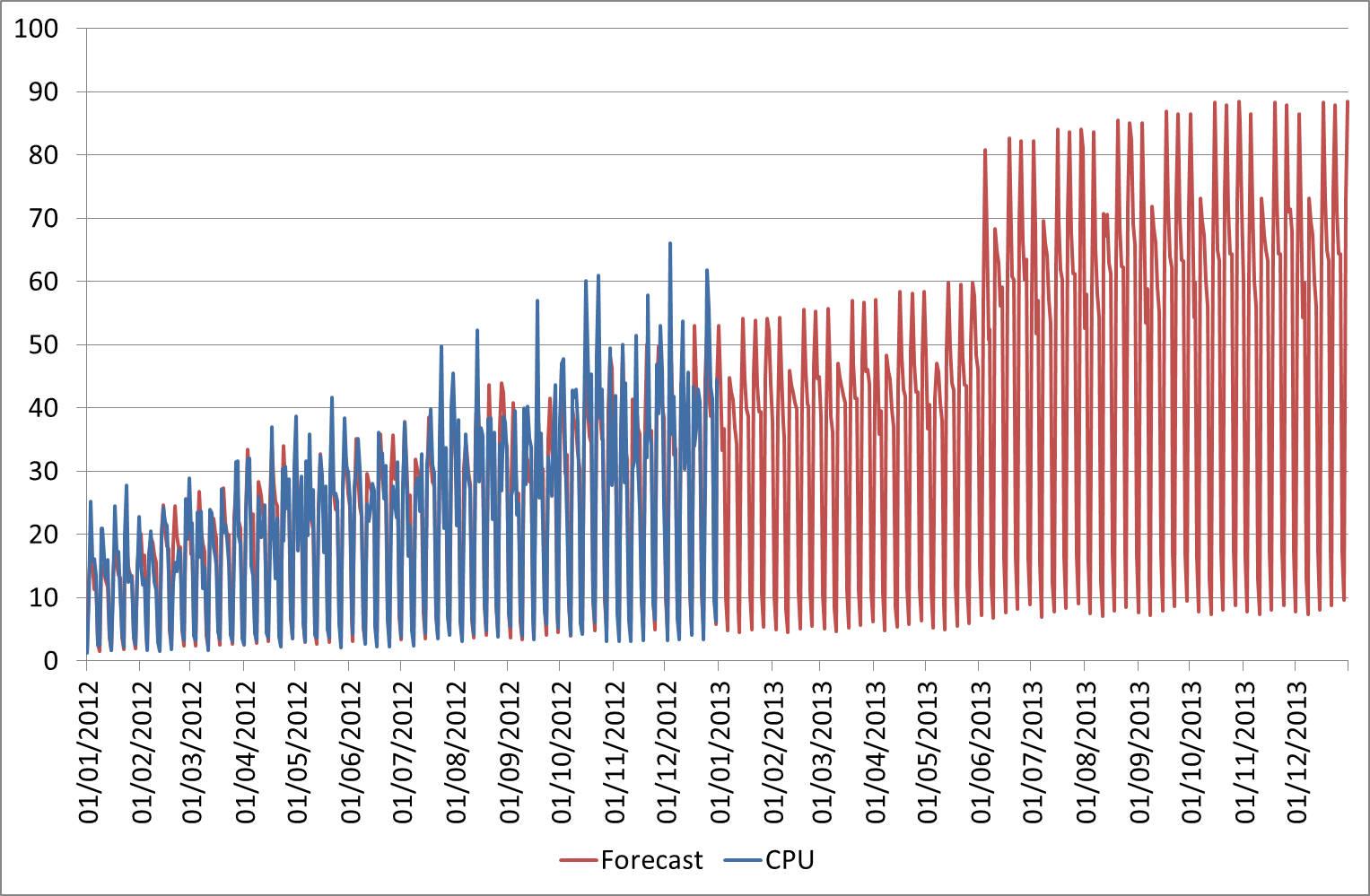
And now the final forecast looks like this:
You can then continue to apply Error etc. to the forecast as discussed in Further Time Series Decomposition in Excel.
As you can see this is quite powerful and we can simply plug in new business volumes to our BusinessData table to get new predictions.

