
In my earlier posts on forecasting with Time Series Decomposition (see Forecasting: Further Time Series Decomposition in Excel) we looked at producing a forecast based on historical behaviour of the data. The forecast we had at the end, including upper bound forecast error, looked like this:
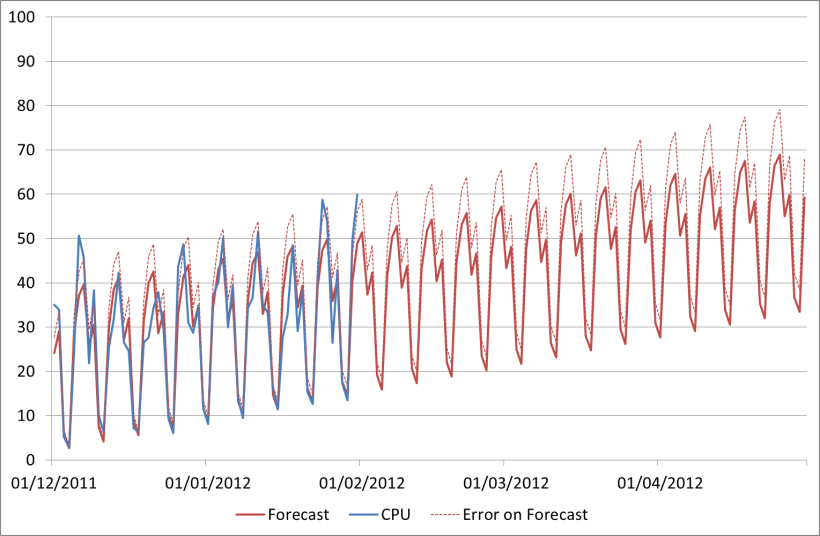
Now this looks great, it gives me a fairly low error and if everything continues in that way it will be fairly accurate. If it does. But what if it doesn’t? I can have all the historical data in the world and build the most complex model of it, but if that assumption is incorrect my forecast is going to be wrong.
Change
The truth of the matter is that things do change. Businesses do expand (or shrink) suddenly. Promotions increase user numbers. New functionality changes user behaviour.
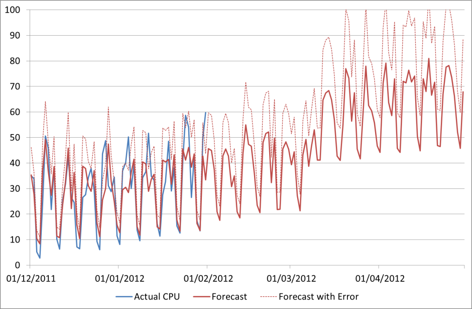
As mentioned before, maybe the actual CPU on our favourite server will look like this:
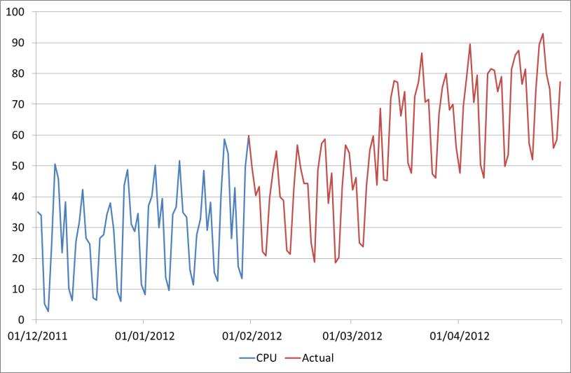
How could we have forecast this from the available data? The answer is we couldn’t. What if we had 10 years’ worth of data going back to 2002? Unless this is a regular uplift that happens e.g. every March, we still couldn’t have predicted it.
But almost certainly, someone knew that change was going to happen. Maybe the business who have been planning that promotion/acquisition/enrolment for months if not years. Maybe the dev team who have finally decided to remove caching to fix that niggling functional bug! This is where we need to be able to put known information into our forecasts so that they are based on more than just historical data.
On the other hand though, the business doesn’t know what effect their decisions will have on our CPU. They know that, due to a new marketing channel, sales are expected to double from March onwards; but it’s our job to work out what impact that will have on the servers. And this is where regression modelling in Excel comes in.
Finding relationships
Let’s assume that someone can give you a data set of historical sales volumes and a forecast for how many sales will be made per day over the next few months. Now there may not be an exact forecast in which case you’ll have to build it from the information available, but that’s another topic.
First let’s graph the sales and CPU together and see if they look similar. As they are different scales we’ll put them on separate axes.
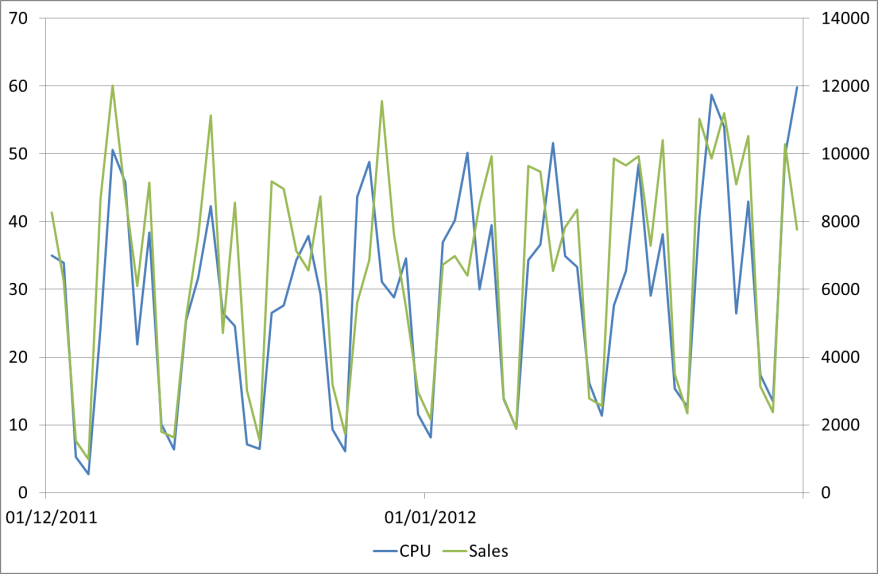
Those look like they follow a similar pattern. To confirm we can do a scatter plot of the relationship between these variables.

We can see there is a relationship here, though with an R2 of just 0.63 perhaps not as strong as we might have hoped. There are other things we could try at this stage such as fitting other reasonable non-linear models, eliminating outliers with known causes, looking at other factors etc. For simplicity though we’ll just use the linear relationship we have identified. The question ‘is this relationship strong enough’ very much comes down to the error tolerance of your forecasts. Some real scenarios will have a much stronger linear relationship particularly when volumes are very large, which means we can have much more confidence in the forecasting results. A good case study of a strong linear regression we’ve seen is with Domino’s pizza orders against CPU load – you can find a graph of this on slide 16 of this presentation which one of our consultants gave recently.
Building the forecast
Here is the forecast we have been given for Sales:
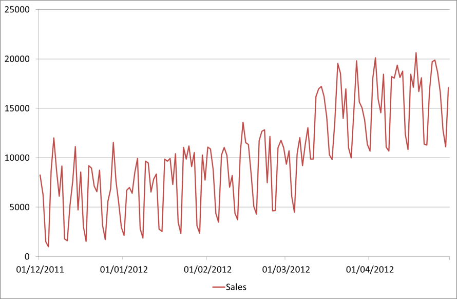
Now we can simply use whatever relationship we found to translate this into CPU.
This is done using the same techniques we used before for linear regression, except here the driver is the sales rather than the date.
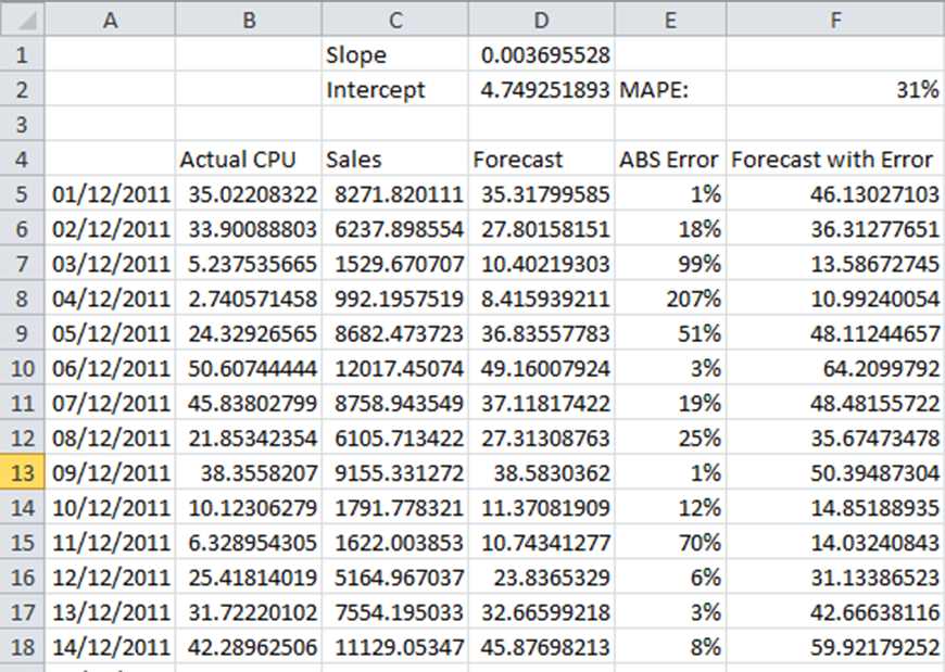
Here the slope is defined as =SLOPE(B5:B66,C5:C66), the intercept as =INTERCEPT(B5:B66,C5:C66)
The forecast CPU is then Sales * Slope + Intercept, e.g. =C5*D$1+D$2
And again we are using an MAPE error figure to identify the upper bounds of the forecast. The error figure of 31% is quite a bit higher than the 15% that we had on the Time Series Decomposition forecast. However what we have sacrificed in fit to historical data we have gained in understanding of future behaviour, which is after all what the forecast is for! If we return to our forecast to validate it with the Actual figures given in the second chart above, we now have an error of 27% on the TSD forecast, but only 12% on the Regression one.

This is because, even though the relationship is not as strong as it might be, we have captured some knowledge of future behaviour into our forecast, and that makes all the difference.
Maybe some more on how to get the business forecasts (and in the right form) another time!

