

Blogs
Date 29 June 2026
Part 3 of Statistics within Capacity Management and Performance Engineering Series.
Having spent the past 2 weeks within the world of probability and distributions a change was necessary. Herein we will be discussing linearization. Let’s assume you have plotted a trend and it is not linear, how can you interpret this and make a prediction from this?
Let’s assume we have a function of one variable (these principles can be expanded for multivariable systems):
(1) ![]()
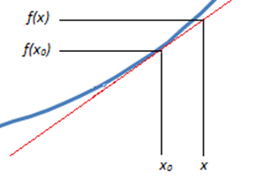
This is easily manipulated within our example. Let us consider a point on the this line (x0,f(x0). We know this point and we want the approximation at (x,f(x)). With this little information we can make a linearization of the curve.
With observation it is clear that the linear approximation then follows the form of:
(2) 
This is rather convenient as it matches the form of a linear function. The approximation is said to be exact at the point at which it is defined (x0,f(x0)). The further from this point the approximation needs to be treated with caution.
Example
(3) 
Using (2) and substituting the values:
(4) 
And now we can simplify:
(5) 
Thus we now have a linear approximation at the point 1,1 for y=x2 using this we can now make an approximation. Let’s assume we want to know what the value of y will be when x is 1.1. The approximation gives 1.2, while the actual value is 1.21. Our approximation falls within 1% of the actual value. This is a powerful tool for making approximations close to a known value. And can provide a good estimate before much more complicated analysis is undertaken.

About the author
Team Capacitas

FinOps and AI: Building the Financial Discipline for the Next Wave of Enterprise Intelligence
AI FinOps represents an evolution rather than a replacement of traditional FinOps. It extends the model into a domain where financial, technical, and product decisions are tightly interconnected. blogs-(new)-post

Confidence Under Load: How We Verified AKS Readiness for Peak
How Capacitas verified AKS readiness for peak demand by validating workload performance, autoscaling, cluster capacity, monitoring, and incident response. blogs-(new)-post
Building Cloud Resilience: Lessons from the AWS Outage
Learning from the Latest Outage. Events like this week’s AWS disruption highlight one clear truth: resilience must be designed, not assumed. blogs-(new)-post

Bringing Order to Chaos: A Practical Guide to Chaos Testing in the Cloud
In today’s cloud-native environments, resilience is not optional—it’s critical. Chaos testing has emerged as a key practice for validating system behaviour under failure conditions. blogs-(new)-post

